One of most
discussed question about TSQL algorithms is „How to transpose (change columns
into rows) a table?” Most solutions based on static code which is adapted to
your table. For every table, you need to write different code. Some
authors propose using PIVOT statement, but it is not very handy to use this
because PIVOT uses rows aggregation so avoiding this is always so
easy.
Another
question is "What if i need not only data change but gets columns/rows names
too?” I you read my previous posts so you know which method we will use:
XML-based. This is how it looks:
DECLARE @xml XML ,
    @RowCount BIGINT
CREATE TABLE #Table
    (
      Column#1 INT ,
      Column2 NVARCHAR(MAX) ,
      Column3 DECIMAL(15, 2)
    )
CREATE TABLE #TempTable
    (
      RowID BIGINT ,
      CellId BIGINT ,
      Value NVARCHAR(MAX) ,
      ColumnName NVARCHAR(MAX)
    )
DECLARE @sSQl NVARCHAR(MAX)= 'SELECT (SELECT DISTINCT ColumnName FROM #TempTable WHERE CellId=Cell.CellId) as ColumnName,'
INSERT  INTO #Table
        SELECT  5 ,
                'Column_1_Test_String' ,
                99.99
INSERT  INTO #Table
        SELECT  9 ,
                'Column_2_Test_String' ,
                NULL


SET @xml = ( SELECT * ,
                    Row_Number() OVER ( ORDER BY ( SELECT   1
                                                 ) ) Rn
             FROM   #Table Row
           FOR
             XML AUTO,
                 ROOT('Root') ,
                 ELEMENTS XSINIL
           ) ;
WITH XMLNAMESPACES('http://www.w3.org/2001/XMLSchema-instance' AS xsi),RC AS
   (SELECT COUNT(Row.value('.', 'nvarchar(MAX)')) [RowCount]
   FROM @xml.nodes('Root/Row') AS WTable(Row))
,c AS(
SELECT b.value('local-name(.)','nvarchar(max)') ColumnName,
  b.value('.[not(@xsi:nil = "true")]','nvarchar(max)') Value,
  b.value('../Rn[1]','nvarchar(max)') Rn,
  ROW_NUMBER() OVER (PARTITION BY b.value('../Rn[1]','nvarchar(max)') ORDER BY (SELECT 1)) Cell
FROM
 @xml.nodes('//Root/Row/*[local-name(.)!="Rn"]') a(b)

 ),Cols AS (
 SELECT  DISTINCT c.ColumnName,
  c.Cell
 FROM c
 )
 INSERT INTO #TempTable (CellId,RowID,Value,ColumnName)
 SELECT Cell,Rn,Value,REPLACE(c.ColumnName,'_x0023_','#')
 FROM c

SELECT  @sSQL = @sSQl
        + '(SELECT T2.Value FROM #Temptable T2 WHERE T2.CellId=Cell.CellID AND T2.Rowid='
        + CAST(T.RowId AS NVARCHAR) + ') AS Row_' + CAST(T.RowID AS NVARCHAR)
        + ','
FROM    ( SELECT DISTINCT
                    RowId
          FROM      #TempTable
        ) T
SET @sSQl = LEFT(@sSQL, LEN(@sSQL) - 1)
    + ' FROM (SELECT DISTINCT CellId FROM #TempTable) Cell'
EXECUTE sp_Executesql @sSQl
--here you will have your output
DROP TABLE #Table
DROP TABLE #TempTable
Description: Lines 1-24: declaring variables and filling up source
table: Lines 25-33: writing source table as XML into XML
variable
Lines 34-52:
filling up ##Temptable (temporary table). It is used for debug purpose only. If
you test this solution, you can avoid this and implement it as next CTE in chain
of sub-queries.
Lines 54-63: Create dynamic SQL statement to prepare
transposed output Line 64: Executing dynamic SQL. Here we have next
output:
Lines 66-67 Dropping temporary
tables.
Here I described how you can easily transpose table
without knowing nothing about source table structure. Based on code above,you
can prepare stored procedure which will get XML generated from table and it will
return transposed XML. In such way you can easily transpose any of your tables
from any place in your code.
A heap is a table without a clustered index. Heaps have one row in sys.partitions, with index_id = 0 for each partition used by the heap. By default, a heap has a single partition. When a heap has multiple partitions, each partition has a heap structure that contains the data for that specific partition. For example, if a heap has four partitions, there are four heap structures; one in each partition.
Depending on the data types in the heap, each heap structure will have one or more allocation units to store and manage the data for a specific partition. At a minimum, each heap will have one IN_ROW_DATA allocation unit per partition. The heap will also have one LOB_DATA allocation unit per partition, if it contains large object (LOB) columns. It will also have one ROW_OVERFLOW_DATA allocation unit per partition, if it contains variable length columns that exceed the 8,060 byte row size limit. For more information about allocation units, see Table and Index Organization.
The column first_iam_page in the sys.system_internals_allocation_units system view points to the first IAM page in the chain of IAM pages that manage the space allocated to the heap in a specific partition. SQL Server uses the IAM pages to move through the heap. The data pages and the rows within them are not in any specific order and are not linked. The only logical connection between data pages is the information recorded in the IAM pages.
The sys.system_internals_allocation_units system view is reserved for Microsoft SQL Server internal use only. Future compatibility is not guaranteed.
Table scans or serial reads of a heap can be performed by scanning the IAM pages to find the extents that are holding pages for the heap. Because the IAM represents extents in the same order that they exist in the data files, this means that serial heap scans progress sequentially through each file. Using the IAM pages to set the scan sequence also means that rows from the heap are not typically returned in the order in which they were inserted.
The following illustration shows how the SQL Server Database Engine uses IAM pages to retrieve data rows in a single partition heap.
Unique and non-unique SQL Server indexes on a heap table
In the upcoming weblog postings I want to work out the differences between unique and non-unique indexes in SQL Server. I assume that you already know the concepts about clustered- and non clustered indexes and how they are used in SQL Server.
In the past I've done a lot of trainings and consulting regarding SQL Server performance tuning and it seems that some people doesn't know the differences and implications between unique and non-unique indexes. And as you will see in the upcoming postings there are really big differences how SQL Server stores those two variants that impact the size and the efficiency of your indexes.
Let's start today with unique and non unique non clustered indexes on a table without a clustered index, a so-called heap table in SQL Server. The following listing shows how to create our test table and populate it with 80.000 records. Each record needs 400 bytes, therefore SQL Server can put 20 records on each data page. This means that our heap table contains 4.000 data pages and 1 IAM page.
-- Create a table with 393 length + 7 bytes overhead = 400 bytes -- Therefore 20 records can be stored on one page (8.096 / 400) = 20,24 CREATETABLE CustomersHeap ( CustomerID INTNOTNULL, CustomerName CHAR(100)NOTNULL, CustomerAddress CHAR(100)NOTNULL, Comments CHAR(189)NOTNULL ) GO
-- Insert 80.000 records DECLARE @i INT= 1 WHILE (@i <= 80000) BEGIN INSERTINTO CustomersHeap VALUES ( @i, 'CustomerName'+CAST(@i ASCHAR), 'CustomerAddress'+CAST(@i ASCHAR), 'Comments'+CAST(@i ASCHAR) )
SET @i += 1 END GO
-- Retrieve physical information about the heap table SELECT*FROMsys.dm_db_index_physical_stats ( DB_ID('NonClusteredIndexStructureHeap'), OBJECT_ID('CustomersHeap'), NULL, NULL, 'DETAILED' ) GO
After the creation of the heap table and the data loading, you can now define a unique and non-unique non-clustered index on the column CustomerID of our heap table. We will define both indexes on the same column so that we can analyze the differences between unique- and non-unique non-clustered indexes.
-- Create a unique non clustered index CREATEUNIQUENONCLUSTEREDINDEX IDX_UniqueNCI_CustomerID ON CustomersHeap(CustomerID) GO
-- Create a non-unique non clustered index CREATENONCLUSTEREDINDEX IDX_NonUniqueNCI_CustomerID ON CustomersHeap(CustomerID) GO
If you want to define a unique non-clustered index on a column that doesn't contain unique data, you will get back an error message from SQL Server. Important to know is that SQL Server creates a non-unique non-clustered index if you don't specify the UNIQUE property when creating a non-clustered index. So by default you will always get a non-unique non-clustered index!
After the creation of both indexes you can analyze their size, their index depth, their size etc. with the DMV sys.dm_db_index_physical_stats. You can to pass in as the 3rd parameter the index-id. The IDs of all non-clustered indexes starts at 2, therefore the first non-clustered index gets the ID 2 and the second one the ID 3
-- Retrieve physical information about the unique non-clustered index SELECT*FROMsys.dm_db_index_physical_stats ( DB_ID('NonClusteredIndexStructureHeap'), OBJECT_ID('CustomersHeap'), 2, NULL, 'DETAILED' ) GO
-- Retrieve physical information about the non-unique non-clustered index SELECT*FROMsys.dm_db_index_physical_stats ( DB_ID('NonClusteredIndexStructureHeap'), OBJECT_ID('CustomersHeap'), 3, NULL, 'DETAILED' ) GO
As you can see from both outputs, the index root page of the unique non-clustered index is occupied of around 24%, where the index root page of the non-unique non-clustered index is occupied of around 39%, so there must be a difference in the storage format of unique/non-unique non-clustered indexes on a heap table! In the next step we create a simple helper table that stores the output of the DBCC IND command. The structure of this helper table is directly taken from the excellent book SQL Server 2008 Internals.
After the creation of this helper table we can dump out all pages that are belonging to our non-clustered indexes to this helper table with the following two calls to DBCC INC in combination with the INSERT INTO statement
-- Write everything in a table for further analysis INSERTINTO sp_table_pages EXEC('DBCC IND(NonClusteredIndexStructureHeap, CustomersHeap, 2)') GO
-- Write everything in a table for further analysis INSERTINTO sp_table_pages EXEC('DBCC IND(NonClusteredIndexStructureHeap, CustomersHeap, 3)') GO
Now we can start analyzing our non-clustered indexes by using the undocumented DBCC PAGE command. To get some information back from DBCC PAGE you have to enable the flag 3604 of DBCC:
DBCC TRACEON(3604) GO
Let's dump out the index root page of our unique non-clustered index by the following command:
DBCC PAGE(NonClusteredIndexStructureHeap, 1, 4192, 3) GO
This will result in the following result in SQL Server Management Studio:
As you can see from this screenshot SQL Server stores the child page of the B-tree where the minimum key of the non-clustered index is located. The child page 4161 contains for example the record with the minimum key of 540 up to the maximum key of 1078. When you dump out the index root page with the dump option 1 you get the byte by byte representation of all index records on the index root page:
DBCC PAGE(NonClusteredIndexStructureHeap, 1, 4192, 1) GO
SQL Server needs here 11 bytes for storing an index row. These 11 bytes are storing the following information:
1 byte: Status Bits
4 bytes: Customer ID, like 540
4 bytes: child PageID, like 4161
2 bytes: FileID, like 1
As you can see it's up to the length of the non-clustered key how long an index row is. This also means that SQL Server is able to store more index rows on an index page if you choose a smaller non-clustered key. If you choose for example a CHAR(100) as a non-clustered index key, then SQL Server needs more index pages for your non-clustered index, which is not so efficient as using a smaller index key. The T-SQL script enclosed to this posting shows you how you can decode those bytes from the hexadecimal representation.
Finally you can dump out the child page 4161, which is located on the leaf-level of the non-clustered index.
DBCC PAGE(NonClusteredIndexStructureHeap, 1, 4161, 3) GO
As you can see from the figure, SQL Server stores for each index key on which data page and on which slot the corresponding record is located. Because we have not defined a clustered index on our table, SQL Server uses here the RID (Row Identifier) to point to the correct record on the data page. Index pages on the leaf-level on a heap table are different from leaf-level index pages defined on a clustered table (a table that contains a clustered index).When you dump out the leaf-level index page of the non-clustered index you can see that SQL Server needs 13 bytes per index row:
1 byte: Status Bits
4 bytes: CustomerID, like 540
4 bytes: PageID, like 178,
2 bytes: FileID, like 1
2 bytes: Slot number, like 19
Finally with this information in your hand, it is very easy to locate the correct record on the data page, because you know the PageID, FileID, and also the slot number where the record on the data page is located. Easy, isn't it?
Let's move on now to non-unique non-clustered indexes. Earlier we have already created such an index, which gets the index-id of 3 from SQL Server, because it's the second non-clustered index we have defined. In my case the index root page of the non-unique non-clustered index is located on page 4264, therefore I dump it out with the following command:
DBCC PAGE(NonClusteredIndexStructureHeap, 1, 4264, 3) GO
But wait! Now the result from DBCC PAGE on the root index page on a non-unique non-clustered index is different! As you can see SQL Server returns here an additional column named "HEAP RID (key)". The value in this column is used to make your non-unique non-clustered index unique. The HEAP RID column uses 8 additional bytes in your index row, which encodes the following information that are granted to be unique on a heap table:
4 bytes: PageID, like 178
2 bytes: FileID, like 1
2 bytes: Slot number, like 19
The overead of a non-unique non-clustered index on a heap table costs you 8 additional bytes per index row - on all index levels, expect the leaf-level, because SQL Server stores here always the HEAP RID as you have seen previously! So please keep this 8 bytes of additional index record overhead in mind, when you create non-clustered indexed that are NOT unique! And as I have said earlier, they are NOT unique by default!!!
In this example your non-unique non-clustered index is about 2 times bigger than the unique non-clustered index, because the unique index needs 11 bytes and the non-unique index needs 19 bytes (overhead of 8 bytes). When you look back to the output of the DMV sys.dm_db_index_physical_stats you can see that the index root page of the unique non-clustered index has a page space usage of around 24% where the index root page of the non-unique non-clustered index has a page space usage of around 39%. This will make a big difference on large non-clustered indexes!
With SQL Server 2012, Microsoft continues its investment in self-service business intelligence (BI) with the introduction of Power View, an interactive, web-based data exploration, visualization, and presentation technology. I'll discuss the underlying architecture of Power View and how it fits into Microsoft's overall BI strategy. I'll then walk you through how to install it and take advantage of its capabilities.
Do We Need Another BI Tool?
Figure 1 illustrates how Power View fits into Microsoft's overall BI strategy. With a BI platform that already includes Microsoft Excel, Excel Services, SQL Server Reporting Services (SSRS), and PerformancePoint Services, you might be wondering why Microsoft introduced another BI tool. Although it does share similarities with these existing technologies, Power View extends ad-hoc reporting to a broader audience.
Figure 1: Understanding how Power View fits into Microsofts overall BI strategy
In most organizations, there are a small number of end users who are comfortable building Excel PivotTables and PivotCharts. Excel Services makes PivotTables easy to consume, but the workbooks published to Excel Services are fairly fixed in terms of layout and interactivity. The number of users who can design a report in SSRS is very small, even with tools such as Report Builder. PerformancePoint Services provides intuitive charts and grids, but their design and deployment is usually done by an IT professional. Plus, there's no easy way for end users to save personal views. Power View not only addresses these important usability gaps but also provides its own unique capabilities.
Installing Power View
Power View is a component of SSRS 2012. Specifically, it's part of SSRS installed in SharePoint integrated mode. To install Power View in your environment, you need SharePoint 2010 Enterprise Edition SP1 or later.
Power View is designed to work against an intermediate, business-friendly tabular data model. This tabular data model can be either a PowerPivot workbook that has been deployed to a SharePoint document library or a database in a SQL Server Analysis Services (SSAS) 2012 instance running in tabular mode. Microsoft plans to support connectivity to SSAS running in multidimensional mode in a future service pack.
Getting Started
Power View reports are created in a web browser. Because Power View leverages Microsoft Silverlight, there's no desktop application for report authors (or consumers) to download, other than the Silverlight 5.0 runtime. Figure 2 shows an example of how to launch Power View from a SharePoint library, using a PowerPivot workbook as the data source. Power View can also be launched by clicking a Report Data Source (RDS) file or a Business Intelligence Semantic Model (BISM) file, a new type of data connection. The RDS or BISM file is stored in a SharePoint document library and points to either a PowerPivot workbook or a tabular mode database.
Figure 2: Launching Power View from a SharePoint library
Once launched, the authoring environment looks and behaves like a cross between Excel, Report Builder, and PowerPoint. Similar to an Excel PivotTable, you can check fields (or drag and drop fields) in a table list to begin building a report, as shown in Figure 3. Another similarity to a PivotTable is that there's no need to switch between design mode and preview mode. Every change made to the report is instantly visible. Note that behind the scenes, Power View communicates with a tabular data model by issuing Data Analysis Expressions (DAX) queries. DAX was initially introduced as an expression language in PowerPivot.
Figure 3: Building a report in Power View
Like Report Builder, Power View has many types of visualizations from which to choose. In my report, I wanted to analyze various economic indicators by presidential term. I selected the Tiles visualization so that each tile represents a president, and I converted the initial table to a card view (which displays each row from a table in a format similar to an index card). A tile acts as a container in that the card and any additional tables and charts will automatically be scoped to the selected tile (in this case, a particular president). Like a traditional reporting tool, Power View lets you arrange different tables and charts in a free-form manner. For example, in Figure 4, I added a line chart within the tile to display economic growth by calendar quarter. In addition to the line chart, Power View supports matrix, column, bar, and scatter charts.
Figure 4: Adding a line chart within the tile to display economic growth by calendar quarter
Saving and Sharing Power View Reports
To save a Power View report, you simply click Save on the File menu. The report is saved as a single file, with an .rdlx extension. A report file can be saved locally, but it must be saved to a SharePoint document library in order for others to view it.
Viewing a saved report is straightforward. An end user simply clicks the report from a document library, and it's rendered in the browser. (Note that a user will need both Read and View permissions to view a Power View report.) From here, the user can print, export, or edit the report. Any user who is able to view a report is also able to edit it, but the user must have at least Contribute permissions to save any changes.
One of the most important routes to high performance in a SQL Server database is the index. Indexes speed up the querying process by providing swift access to rows in the data tables, similarly to the way a book’s index helps you find information quickly within that book. In this article, I provide an overview of SQL Server indexes and explain how they’re defined within a database and how they can make the querying process faster. Most of this information applies to indexes in both SQL Server 2005 and 2008; the basic structure has changed little from one version to the next. In fact, much of the information also applies to SQL Server 2000. This does not mean there haven’t been changes. New functionality has been added with each successive version; however, the underlying structures have remained relatively the same. So for the sake of brevity, I stick with 2005 and 2008 and point out where there are differences in those two versions.
Index Structures
Indexes are created on columns in tables or views. The index provides a fast way to look up data based on the values within those columns. For example, if you create an index on the primary key and then search for a row of data based on one of the primary key values, SQL Server first finds that value in the index, and then uses the index to quickly locate the entire row of data. Without the index, a table scan would have to be performed in order to locate the row, which can have a significant effect on performance.
You can create indexes on most columns in a table or a view. The exceptions are primarily those columns configured with large object (LOB) data types, such as image, text, and varchar(max). You can also create indexes on XML columns, but those indexes are slightly different from the basic index and are beyond the scope of this article. Instead, I'll focus on those indexes that are implemented most commonly in a SQL Server database.
An index is made up of a set of pages (index nodes) that are organized in a B-tree structure. This structure is hierarchical in nature, with the root node at the top of the hierarchy and the leaf nodes at the bottom.
Clustered Indexes
A clustered index stores the actual data rows at the leaf level of the index. Returning to the example above, that would mean that the entire row of data associated with the primary key value of 123 would be stored in that leaf node. An important characteristic of the clustered index is that the indexed values are sorted in either ascending or descending order. As a result, there can be only one clustered index on a table or view. In addition, data in a table is sorted only if a clustered index has been defined on a table.
Note: A table that has a clustered index is referred to as a clustered table. A table that has no clustered index is referred to as a heap
Nonclustered Indexes
Unlike a clustered indexed, the leaf nodes of a nonclustered index contain only the values from the indexed columns and row locators that point to the actual data rows, rather than contain the data rows themselves. This means that the query engine must take an additional step in order to locate the actual data.
A row locator’s structure depends on whether it points to a clustered table or to a heap. If referencing a clustered table, the row locator points to the clustered index, using the value from the clustered index to navigate to the correct data row. If referencing a heap, the row locator points to the actual data row.
Nonclustered indexes cannot be sorted like clustered indexes; however, you can create more than one nonclustered index per table or view. SQL Server 2005 supports up to 249 nonclustered indexes, and SQL Server 2008 support up to 999. This certainly doesn’t mean you should create that many indexes. Indexes can both help and hinder performance, as I explain later in the article.
In addition to being able to create multiple nonclustered indexes on a table or view, you can also add included columns to your index. This means that you can store at the leaf level not only the values from the indexed column, but also the values from non-indexed columns. This strategy allows you to get around some of the limitations on indexes. For example, you can include non-indexed columns in order to exceed the size limit of indexed columns (900 bytes in most cases).
Index Types
In addition to an index being clustered or nonclustered, it can be configured in other ways:
Composite index: An index that contains more than one column. In both SQL Server 2005 and 2008, you can include up to 16 columns in an index, as long as the index doesn’t exceed the 900-byte limit. Both clustered and nonclustered indexes can be composite indexes.
Unique Index: An index that ensures the uniqueness of each value in the indexed column. If the index is a composite, the uniqueness is enforced across the columns as a whole, not on the individual columns. For example, if you were to create an index on the FirstName and LastName columns in a table, the names together must be unique, but the individual names can be duplicated.
A unique index is automatically created when you define a primary key or unique constraint:
Primary key: When you define a primary key constraint on one or more columns, SQL Server automatically creates a unique, clustered index if a clustered index does not already exist on the table or view. However, you can override the default behavior and define a unique, nonclustered index on the primary key.
Unique: When you define a unique constraint, SQL Server automatically creates a unique, nonclustered index. You can specify that a unique clustered index be created if a clustered index does not already exist on the table.
Covering index: A type of index that includes all the columns that are needed to process a particular query. For example, your query might retrieve the FirstName and LastName columns from a table, based on a value in the ContactID column. You can create a covering index that includes all three columns.
Index Design
As beneficial as indexes can be, they must be designed carefully. Because they can take up significant disk space, you don’t want to implement more indexes than necessary. In addition, indexes are automatically updated when the data rows themselves are updated, which can lead to additional overhead and can affect performance. As a result, index design should take into account a number of considerations.
Database
As mentioned above, indexes can enhance performance because they can provide a quick way for the query engine to find data. However, you must also take into account whether and how much you’re going to be inserting, updating, and deleting data. When you modify data, the indexes must also be modified to reflect the changed data, which can significantly affect performance. You should consider the following guidelines when planning your indexing strategy:
For tables that are heavily updated, use as few columns as possible in the index, and don’t over-index the tables.
If a table contains a lot of data but data modifications are low, use as many indexes as necessary to improve query performance. However, use indexes judiciously on small tables because the query engine might take longer to navigate the index than to perform a table scan.
For clustered indexes, try to keep the length of the indexed columns as short as possible. Ideally, try to implement your clustered indexes on unique columns that do not permit null values. This is why the primary key is often used for the table’s clustered index, although query considerations should also be taken into account when determining which columns should participate in the clustered index.
The uniqueness of values in a column affects index performance. In general, the more duplicate values you have in a column, the more poorly the index performs. On the other hand, the more unique each value, the better the performance. When possible, implement unique indexes.
For composite indexes, take into consideration the order of the columns in the index definition. Columns that will be used in comparison expressions in the WHERE clause (such as WHERE FirstName = 'Charlie') should be listed first. Subsequent columns should be listed based on the uniqueness of their values, with the most unique listed first.
You can also index computed columns if they meet certain requirements. For example, the expression used to generate the values must be deterministic (which means it always returns the same result for a specified set of inputs).
Fulltext Search codebase has been significantly revamped to address both query performance and throughput on large scale (millions of documents) with concurrent updates. With SQL2008 they moved all the index storage in the database file and majority of population logic in to the core engine to make fulltext search an integral and fully manageable engine component. However there was work to be done to make it perform and scale against best of the fulltext engines out there in the industry. With Denali CTP1, they are pleased to deliver this improvement.
they looked at the entire code base from how queries block while waiting an ongoing index update to release a shared schema lock, from how much memory is allocated during index fragment population, to how they could reorganize the query code base as a streaming Table Value Function to optimize for TOP N search queries, how they could maintain key distribution histograms to execute search on parallel threads, all the way to how they could take better advantage of the processor compute instructions (scoring ranks for example)… End result is that they are able to significantly boost performance (10X in many cases when it comes to concurrent index updates with large query workloads) and scale without having to change any storage structures or existing API surface. All our customers going from SQL 2008 / R2 to Denali will benefit with this improvement.
Besides performance and scale improvement, they also added support for property scoped searches over documents with file system properties stored with-in a fulltext enabled table. One can now issue a CONTAINS query looking for all documents containing a particular term and authored by a particular author without having to maintain a separate column for the Author name in the database.
they also improved NEAR operator in the CONTAINS predicate to allow users to specify distance between two terms and if the order of the term matters. It is important to note that distances between two words in a single sentence are much smaller compared to the same across two sentences (even if words are placed next to each other with a period in between), or across paragraphs, or across bullet points or across spreadsheet columns or worksheets.
A SQL Server FileTable is a special table where you can store directory and files – that’s not special I know, the special thing is that you can access these files and directories from windows applications as if they were stored in the file system.
The data stored in the FileTable is exposed to windows through a windows share, and via this share it is possible to gain non-transactional access to the data.
If you create or change a file through the windows share the command is intercepted by a SQL Server component and the changes are applied to the corresponding data in the FileTable.
First we need to enable the FILE STREAM in SQL Server instance level. Follow the below mentioned steps.
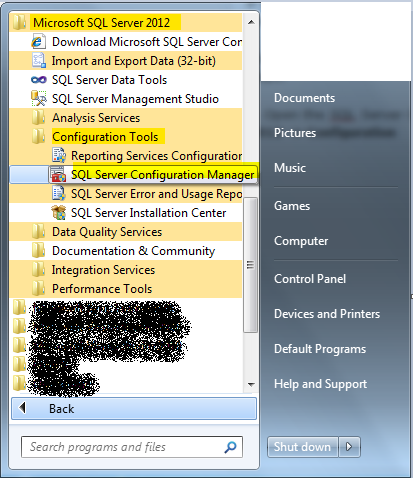
1. Open the SQL Server Configuration Manager by Start -> All Programs -> Microsoft SQL Server 2012 -> Configuration Tools -> SQL Server Configuration Manager
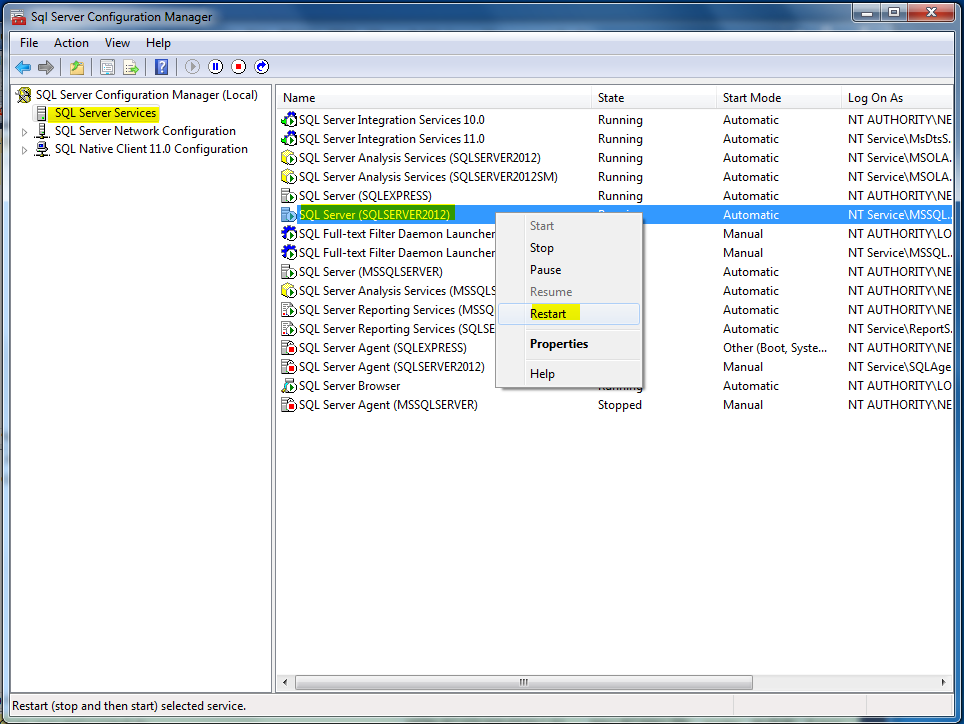
2. Right click on the SQL Server instance under the SQL Server Services menu and select Properties.
3. SQL Server Instance Properties window will be opened. Select the FILESTRAEM tab and tick the below mentioned checkboxes and then click apply and ok
Enable FILESTREAM for Transact-SQL access
Enable FILESTREAM for file I/O access
Allow remote clients access to FILESTREAM data
4. Execute the below mentioned Transact-SQL code in the SSMS.
EXEC sp_configure filestream_access_level, 2
RECONFIGURE
5. Restart the SQL Server Instance.
Let’s create a demo database with a FILESTREAM filegroup, I’ll be setting the NON_TRANSACTED_ACCESS to FULL this gives me full non-transactional access to the share, this option can be changed later if you want to do that. Here is the code:
CREATE DATABASE MyFileTableTest
ON PRIMARY
(
NAME = N'MyFileTableTest',
FILENAME = N'G:\Demo\MyFileTableTest.mdf'
),
FILEGROUP FilestreamFG CONTAINS FILESTREAM
(
NAME = MyFileStreamData,
FILENAME= 'G:\Demo\Data'
)
LOG ON
(
NAME = N'MyFileTableTest_Log',
FILENAME = N'G:\Demo\MyFileTableTest_log.ldf'
)
WITH FILESTREAM
(
NON_TRANSACTED_ACCESS = FULL,
DIRECTORY_NAME = N'FileTable'
)
That’s the database done, now let’s create the magic table – that is simple done with the “AS FileTable” keyword. When creating a FileTable there is only two options that you can change, everything else is out of the box. Let’s have a look at how I created the table:
USE MyFileTableTest
go
CREATE TABLE MyDocumentStore AS FileTable
WITH
(
FileTable_Directory = 'MyDocumentStore',
FileTable_Collate_Filename = database_default
);
GO
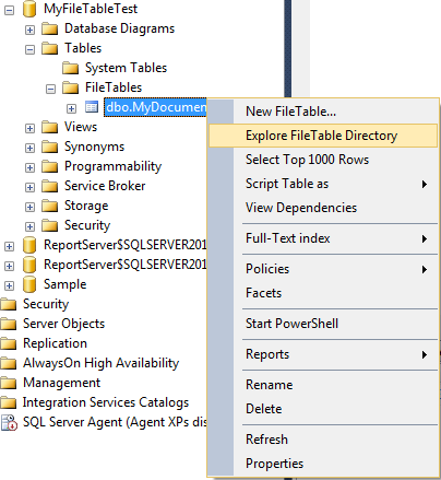
If we take a look at the GUI after creating the table, we can see that the table is created under the new folder called FileTables
that is not the only new thing, if we right click at the table that we just created we will see an option called “Explore FileTable Directory” – click that and a windows opens with the content of your FileTable.
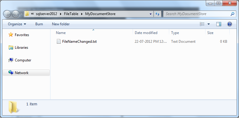
If you drop a file into this folder it will be accessible from SSMS, with a simple SELECT from the MyDocumentStore.
Here is how the folder looks:
And if you query the table you get the following: (This query only shows a few of the columns off the table)
Now you can do file manipulation with SSMS, something like renaming the files is just an update statement
UPDATE MyDocumentStore
SET name = 'FileNameChanged.txt'
WHERE stream_id = 'A124C74D-CCD3-E111-87F1-0019D1EE2D0C'
SSIS is not just about control flows and dataflows, there are other options available in SSIS which extends functionality of SSIS package, and provides a great flexibility in desiging a successfull ETL solution. Lets take a deep insight of what are those options and how we can take benefit of them.
There are four options which extends functionality of SSIS packages.
1. Event Handlers 2. Variables 3. Expressions 4. SQL Queries In this post i will be covering Event handlers, and in later series i will cover Variables, Expressions and SQL queries Event Handlers:
Like any programming languages (C# or JAVA) SSIS also provides Event handlers, which provides functionality of performing some task on a specific event during runtime. At runtime of any SSIS task, series of event takes place, and SSIS Desginer has provided with one tab (Event Handler) to program any action that can be performed on occurance of that event.
Event handlers are created in the same manner as control flow but in different tab as shown.
How we create events?
Its as simple as creating control flow of package.
1. Select the executable container to which the handler will be assigned. 2. Select the event to which you wish the event handler to react to. 3. Drag control flow container and task and connect them together with precedence constraints.
How Events are actually gets handled in SSIS?
Events can be handled at task or container or package level, following is the order it will be handled.
1. Task 2. Container 3. Package
For example: If an event is triggered at the task level and no event handler is defined, the event is passed to container level, if no event handler is defined at container level then it will be passed to package level.
How many events are available?
There are 12 different events that can be handled in SSIS package. Below is the list..
OnError The OnError event is caused by the occurrence of an error.
OnExecStatusChanged The OnExecStatusChanged event occurs when an executable changes its status.
OnInformation When an executable reports information during validation or execution, the OnInformation event occurs.
OnPostExecute OnPostExecute is an event that occurs immediately after an executable has completed running.
OnPostValidate The OnPostValidate event occurs immediately after an executable has finished its validation.
OnPreExecute The OnPreExecute event occurs immediately before an executable runs.
OnPreValidate The OnPreValidate event occurs immediately before an executable begins its validation.
OnProgress OnProgress is an event that occurs when an executable makes measurable progress.
OnQueryCancel The OnQueryCancel event occurs automatically at regular intervals to determine if the package should continue running.
OnTaskFailed When a task has failed execution, the OnTaskFailed event occurs.
OnVariableValueChanged The OnVariableValueChanged event occurs when a variable's value is changed.
OnWarning The OnWarning event is raised when a warning occurs.
Event handlers have a number of properties that allow you to • assign a name and description to the event handler • enable or disable the event handler • determine whether the package fails if the event handler fails • determine the number of errors that can occur before the event handler fails • override the execution result that would normally be returned at runtime • determine the transaction isolation level for operations performed by the event handler, and • determine the logging mode used by the event handler